Generating an OSM-EIRENE Plasma Background
Note
This tutorial includes multiple downloadable files, such as data, grids, etc. Links are included where they are needed or you can download all the files ahead of time here:
Starting a run
Now we are ready to generate a plasma background using OSM-EIRENE. The process involves building up an input file from nothing and gradually adding various layer of complexity that are required to obtain agreement with experimental data. To begin, we will generate a meaningless background plasma just to demonstrate the workflow.
First download the grid made by the extended grid generator and place it in your [iris username]/shots directory (e.g., with Filezilla). Using your favorite text editor, such as geany, open up a blank document on iris. Add the following lines and save the document as d3d-167196-osm-v1.d6i within your data directory:
$
$ Required to indicate extended grid generated by Fuse.
$
'{GRID FILE}      File name of the fluid grid to be loaded'  'fort.4'
'{GRID FORMAT}                                            '  2
'{EXIT}'
$
$ Plasma background options
$
'*S21  SOLTEST 0 run normally, -1 test SOL opt            ' -1
Lines the start with a $ are comments and ignored by OEDGE. The first three lines that involve options in { } brackets are specific to extended grids. We will not cover these types of options anymore in this tutorial beyond just mentioning they are needed for grids made with the fuse grid generator. The rest of the input options take the form seen in in option S21. See the following note.
Note
Anatomy of an input option
The most basic input options consist of three things: A tag, a description, and a value. In the above, the tag is *S21, the description is “SOLTEST 0 run normally, -1 test SOL opt” and the value is -1. Every input option has a unique tag and the description is arbitrary and used only to make the input file human-readable. All the input options can be found on this website at Input Options. For instance, documentation for the grid option is found at S21.
Save the input file. The general run command for OEDGE on iris is as follows:
$ ./rundiv_master.sh <DIV input file> <OUT input file> <geometry file name> <fluid plasma filename extension - optional> <CFD solution - optional> <DIVIMP solution - optional>"
For our specific instance, we run by replacing the unused files with “none”:
$ ./rundiv_master.sh d3d-167196-osm-v1 none grid_d3d_167196_3000_v1 none none none
This command submits the run using the slurm scheduler on iris. You can track the status of your jobs by typing wq at the terminal. The progress of the simulation can be tracked by opening up the d3d-167196-osm-v1.output text file.
If you check your output file, you probably got an error having to do with libgfortran. This is because the default gcc compiler that is loaded on iris is ancient, so we need to make sure we load a more modern compiler. The most strtaightforward way to do this is:
$ module purge
$ module load gcc-9.2.0
Run OEDGE again, it should work this time.
To recap our progress to this point:
We created a barebones input file and told OEDGE that we are using an extended grid
We set input option S21 = -1. Following the link to the documentation for S21 tells us that only a plasma background is being generated (via OSM-EIRENE). Tracking impurities via DIVIMP is not performed when this is set to -1.
We saved our input file and submitted it to iris and looked at the output in the
.outputfile.
Once the run is finished, we need to visualize the results. This is covered in the next section.
Visualizing results
All OEDGE results are stored in the results folder. For our purposes, we only need the .dat and .nc files. The first is a human-readable summary of the simulation, and the latter is a NetCDF file containing the data. Copy these two files into the same directory to your own local machine using a file transfer service of your choice (instructions using Filezilla with the fusion VPN here).
Open up the plotting GUI, click Browse… for the NetCDF file and find your .nc file. From the dropdown you can select various quantities to make a 2D plot from, assuming these quantites were calculated in the simulation. So Electron Temperature will generate a 2D plot, but Impurity Density will throw an error since we did not run DIVIMP. The Plot Options… Dialogue allows you to change some of the plot settings such as the colorbar scale or to plot a specific charge state for plot options that allow it. A 2D plot of the plasma density is shown below.
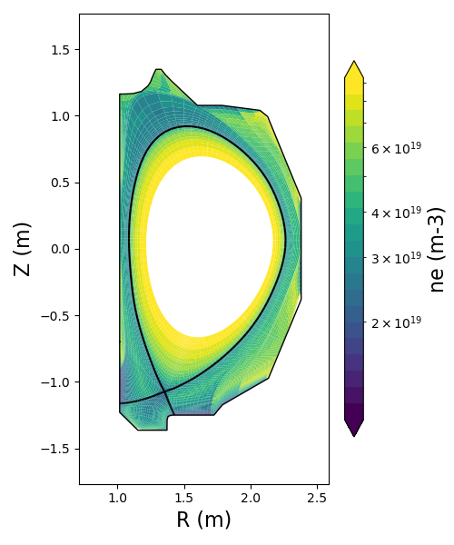
Any of the 2D quantities can also be plotted along a specific “ring”. A ring represents a given flux surface of the grid in the poloidal plane. For example, say we wanted to plot the variation of the electron temperature along the first ring outside of the core. This would be ring number 16 as mentioned in the message box of the GUI. Select Electron Temperature from the dropdown, enter 16 in the Along Ring box and press the corresponding Plot button next to Along Ring.
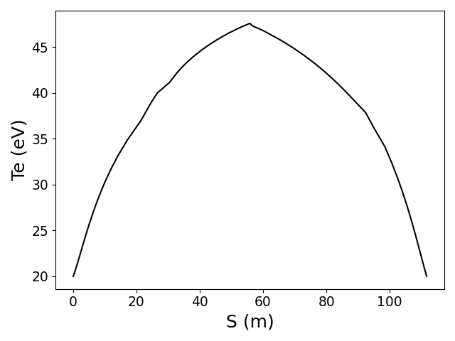
The electron temperature is plotted against the parallel distance along the field line, S. S=0 corresponds to either the inner our outer target. Figuring this out generally becomes clear during the plasma constraning process, but for this example S=0 is the inner target. We will not go into details with the rest of the GUI options as any further functionality is best explored by calling the plotting functions from within custom python scripts. More on that later.
Adding experimental data to OSM
So far, our simulation was ran with default values for hundreds of other input options. Fortunately, we do not need to worry about most of these options and only a subset are needed for making a reliable plasma background. The first step of any OSM background is passing in the available Langmuir probe data. We will use Langmuir probe data from an identical discharge, #167195, because the outer strike point was swept back and forth between 4,000-5,000 ms to fill in the Langmuir probe data for all the flux surfaces. This is very common in well-designed experiments.
The goal is to load the Langmuir probe data and identify which flux surface, or ring, the data is applicable to. You are free to approach this however you’d like, but a simple helper script is included within the repository at python-plots/map_lps_to_grid.py. On your own machine, you can call the script as such:
$ python map_lps_to_grid.py 167195 4000 5000 /path/to/file.nc
Where /path/to/file.nc is the full path to the NetCDF file from above. This has only been tested assuming you are connected through the fusion VPN (sorry for those without it). I fyou are not on the VPN, you can open up a second terminal on your computer and link it to atlas, then set With the above command, the script will output the probe number and label of each probe. It falls onto the user to figure out where each probe is located in the machine (Langmuir probe naming convention has changed throughout the years, which combined with all the possible plasma shapes on DIII-D makes it nearly impossible to automate this process). For this example, probes 23, 25, 29, 31, 33, 35, 51 and 53 are on the outer target and 131 is on the inner target. We call the script again and pass in the locations of each probe to perform the mapping:
python map_lps_to_grid.py 167195 4000 5000 /path/to/file.nc -o 23 25 29 31 33 35 51 53 -i 131 -n 5
The option -n 5 is just to lower the threshold for how many data points in needed in a ring to output the average value for. Within the directory a file 167195_4000_5000.csv is created with the desired data. You may open this up in Excel to help visualize what the data include. A plot of the electron temperature with rings number is shown below.
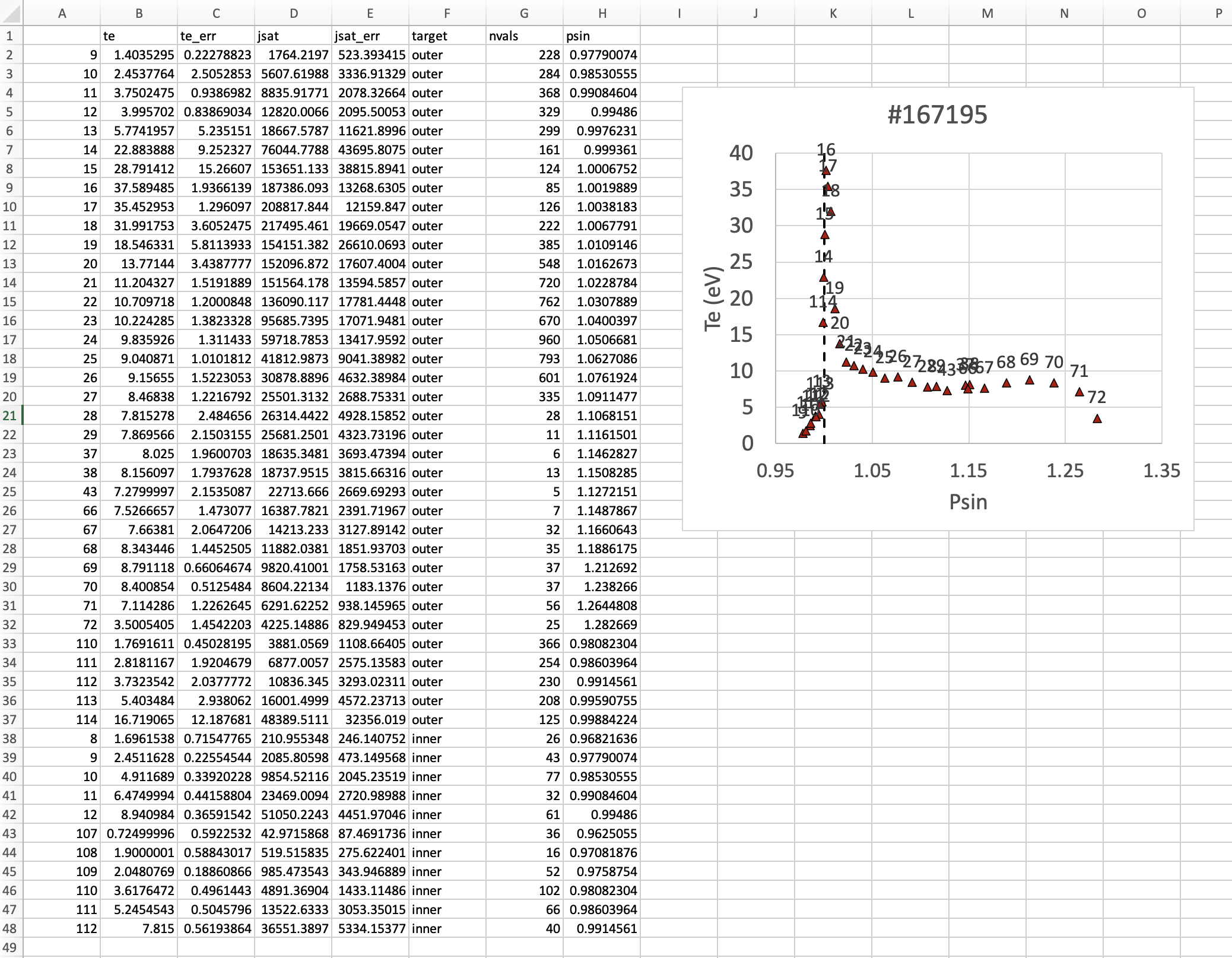
Note that instead of plasma density we are outputting the saturation current, jsat. OEDGE accepts either, but jsat is preferable (see input option Q32). There is significantly less data available for the inner target. In fact, when we plug this into our input file we will actually copy the outer target data for the inner. This is a common approach within OEDGE and is fine as long as your study does not focus on the inner target. But before we do this, we need to gather data for the core.
For this tutorial we use OMFITprofiles to get the core data from Thomson scattering because of the advanced data filtering and fitting tools within it. A tutorial on OMFITprofiles is beyond the scope of this tutorial. The data is exportable in a NetCDF format. You can download the needed NetCDF file for this tutorial here. The following helper script, also located in python-plots/oedge will create a csv file with the required information.
$ python map_omfitprof_to_grid.py 2500 5000 /path/to/oedgefile.nc /path/to/omfitfile.nc
A file called omfit_mapped_to_oedge.csv is created in the same directory. The core temperature data plotted against psin with the ring numbers above each data point is shown below.

We are now ready to copy/paste our mapped data into our input file. The outer and inner target data is passed in via options Q34 and Q35, respectively. The syntax for the input file is as follows:
'*P03 Plasma Decay Option  4=Data input at targets        '  4
'*Q32 Langmuir Probe Switch     0=ne  1=jsat              '  1
'*Q34 ' 'Probe data at outer target                       '
' ' '    Probe data at outer target (dummy line)          '
' Ring     Te      Ti    ne/jsat          Number of rows: '  38
    16  28.16   28.16   1.51E+05
    17  37.59   37.59   1.87E+05
    18  35.45   35.45   2.09E+05
    19  31.99   31.99   2.17E+05
    20  18.55   18.55   1.54E+05
    21  13.77   13.77   1.52E+05
    22  11.20   11.20   1.52E+05
    23  10.71   10.71   1.36E+05
    24  10.22   10.22   9.57E+04
    25  9.84    9.84    5.97E+04
    26  9.04    9.04    4.18E+04
    27  9.16    9.16    3.09E+04
    28  8.47    8.47    2.55E+04
    29  7.82    7.82    2.63E+04
    30  7.87    7.87    2.57E+04
    38  8.03    8.03    1.86E+04
    39  8.16    8.16    1.87E+04
    44  7.28    7.28    2.27E+04
    67  7.53    7.53    1.64E+04
    68  7.66    7.66    1.42E+04
    69  8.34    8.34    1.19E+04
    70  8.79    8.79    9.82E+03
    71  8.40    8.40    8.60E+03
    72  7.11    7.11    6.29E+03
    73  3.50    3.50    4.23E+03
    103 1.00    1.00    1.00E+03  # Manually added for missing PFZ data
    104 1.00    1.00    1.00E+03  #
    105 1.00    1.00    1.00E+03  #
    106 1.00    1.00    1.00E+03  #
    107 1.00    1.00    1.00E+03  #
    108 1.00    1.00    1.00E+03  #
    109 1.00    1.00    1.00E+03  #
    110 1.38    1.38    1.37E+03
    111 1.74    1.74    3.42E+03
    112 2.61    2.61    6.14E+03
    113 3.80    3.80    1.04E+04
    114 4.74    4.74    1.45E+04
    115 16.94   16.94   4.95E+04
'*Q36 ' 'Probe data at inner target                       '
' ' '    Probe data at inner target (dummy line)          '
' Ring     Te      Ti    ne/jsat          Number of rows: '  38
[same as above, inner = outer]
We have assumed \(T_e\) = \(T_i\). We added switch P03 “Plasma Decay Option”. There are historical reasons for this name, but long story short setting this to 4 tells OEDGE to look for the target conditons for each ring from option Q34. We also added Q32 to tell OEDGE we have input the jsat values instead of ne. Note we also manually added data for the PFZ (rings 103-115, see .dat file for ring numbers in each region). The core data is passed in as follows:
'*P02 Core Data Option  1=Input for each ring (Q37)       '  1
'*Q37 ' 'CORE Plasma Data                                 '
' ' '    Core plasma data (dummy line)                    '
'Ring       Te        Ti         ne    Vb  Number of rows:'  15
    1   461.96    461.96   2.58E+19     0
    2   461.96    461.96   2.58E+19     0
    3   384.40    384.40   2.46E+19     0
    4   323.06    323.06   2.32E+19     0
    5   269.25    269.25   2.18E+19     0
    6   229.03    229.03   2.06E+19     0
    7   199.53    199.53   1.94E+19     0
    8   166.73    166.73   1.76E+19     0
    9   135.62    135.62   1.59E+19     0
   10   110.34    110.34   1.47E+19     0
   11    91.47     91.47   1.38E+19     0
   12    78.20     78.20   1.31E+19     0
   13    69.15     69.15   1.25E+19     0
   14    63.39     63.39   1.21E+19     0
   15    59.78     59.78   1.19E+19     0
The core data contains an extra column of the parallel velocity if that data is available, but this is generally optional and not critical so we set it to 0 (this data could be obtained via CER for those who are dedicated). We added switch P02 and set it equal to 1. Like above, this just tells OEDGE to look for the data for core rings in input option Q37. Data in the core region is constant along each ring, though some of the other options for P02 enable some variation along the ring if desired.
Save the input file and run using the same command. Re-running without changing the filename will overwrite all the previous files and helps cut down on storage needs.
Now that we have a SOL solution built using the target Langmuir probe data, we need to compare it to other experimental data within the SOL. This generally means the “upstream” Thomson scattering data, but we also have reciprocating Langmuir probe (RCP) data at the outer midplane as well. To begin, we use the “fastTS” module in OMFIT to get the Thomson scattering data because it has ELM filtering capabilities (not needed for this discharge). Running with default values seems to be appropriate for this discharge. Copy/paste the following code into the Command Box within OMFIT:
import pickle
import numpy as np
from os.path import expanduser

root = OMFIT['fastTS']['OUTPUTS']['current']['filtered_TS']
shot = int(OMFIT['fastTS']['OUTPUTS']['current']['filtered_TS']['shot'])

output = {}
for sysname in ["core", "divertor", "tangential"]:
    sys = root[sysname]
    tmp = {}
    tmp["time"] = np.array(sys["time"])
    tmp["r"] = np.array(sys["r"])
    tmp["z"] = np.array(sys["z"])
    tmp["te"] = np.array(sys["temp"])
    tmp["ne"] = np.array(sys["density"])
    tmp["te_err"] = np.array(sys["temp_e"])
    tmp["ne_err"] = np.array(sys["density_e"])
    tmp["psin"] = np.array(sys["psin_TS"])
    tmp["chord"] = np.array(sys["chord_index"])

    output[sysname] = tmp

home = expanduser("~")
fname = "{}/ts_{}.pickle".format(home, shot)
with open(fname, "wb") as f:
    pickle.dump(output, f)
This saves the Thomson data as a pickled python dictionary in a file called ts_167195.pickle in your home directory. You can download it here.
The RCP data from 167195 can be downloaded here.
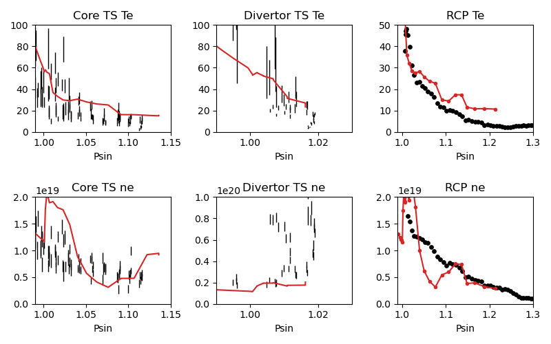
We will use the oedge_plots module to extract the \(n_e\) and \(T_e\) data from the simulation along the path of the Thomson scattering and RCP locations and compare to the respective experimental data. A script demonstrating this is shown below:
import oedge_plots
import pickle
import matplotlib.pyplot as plt
import numpy as np
import pandas as pd

# Load Thomson scattering data.
corets_shift = 0.0
ts_path = "/Users/zamperini/Documents/d3d_work/divimp_files/oedge_tutorial/ts_167195.pickle"
with open(ts_path, "rb") as f:
    ts = pickle.load(f)
ts_plot = {"core": {}, "divertor": {}, "tangential": {}}
for sys in ts.keys():
    tmp = ts[sys]
    mask = np.logical_and(tmp["time"] >= 2500, tmp["time"] <= 5000)
    ts_plot[sys]["time"] = tmp["time"][mask]
    for key in ["te", "te_err", "ne", "ne_err", "psin"]:
        if sys == "core" and key == "psin":
            ts_plot[sys][key] = tmp[key][:, mask] + corets_shift
        else:
            ts_plot[sys][key] = tmp[key][:, mask]
    ts_plot[sys]["chord"] = tmp["chord"]

# Load the RCP data. Data has already been shifted inward by 1.5 cm due to EFIT uncertainties.
rcp_path = "/Users/zamperini/Documents/d3d_work/divimp_files/oedge_tutorial/rcp_156195_2.csv"
rcp = pd.read_csv(rcp_path)

# Load OEDGE run and extract a series of profiles along the locations of TS and RCP.
op_path = "/Users/zamperini/Documents/d3d_work/divimp_files/oedge_tutorial/d3d-167196-osm-v1.nc"
op = oedge_plots.OedgePlots(op_path)
op_tsc_te = op.along_line(1.94, 1.94, 0.67, 0.85, "KTEBS", "psin")
op_tsc_ne = op.along_line(1.94, 1.94, 0.67, 0.85, "KNBS", "psin")
op_tsd_te = op.along_line(1.484, 1.484, -0.82, -1.17, "KTEBS", "psin")
op_tsd_ne = op.along_line(1.484, 1.484, -0.82, -1.17, "KNBS", "psin")
op_rcp_te = op.along_line(2.18, 2.30, -0.188, -0.188, "KTEBS", "psin")
op_rcp_ne = op.along_line(2.18, 2.30, -0.188, -0.188, "KNBS", "psin")

# Now we do our comparison plots.
fig, ((ax1, ax2, ax3), (ax4, ax5, ax6)) = plt.subplots(2, 3, figsize=(8, 5))

# Core TS Te.
x = ts_plot["core"]["psin"].flatten()
y = ts_plot["core"]["te"].flatten()
yerr = ts_plot["core"]["te_err"].flatten()
ax1.errorbar(x, y, yerr, elinewidth=1, ecolor="k", color="k", markersize=15, lw=0)
ax1.plot(op_tsc_te["psin"], op_tsc_te["KTEBS"], color="tab:red")
ax1.set_xlabel("Psin")
ax1.set_title("Core TS Te")
ax1.set_xlim([0.99, 1.15])
ax1.set_ylim([0, 100])

# Core TS ne.
x = ts_plot["core"]["psin"].flatten()
y = ts_plot["core"]["ne"].flatten()
yerr = ts_plot["core"]["ne_err"].flatten()
ax4.errorbar(x, y, yerr, elinewidth=1, ecolor="k", color="k", markersize=15, lw=0)
ax4.plot(op_tsc_ne["psin"], op_tsc_ne["KNBS"], color="tab:red")
ax4.set_xlabel("Psin")
ax4.set_title("Core TS ne")
ax4.set_xlim([0.99, 1.15])
ax4.set_ylim([0, 2.0e19])

# Divertor TS Te
x = ts_plot["divertor"]["psin"].flatten()
y = ts_plot["divertor"]["te"].flatten()
yerr = ts_plot["divertor"]["te_err"].flatten()
ax2.errorbar(x, y, yerr, elinewidth=1, ecolor="k", color="k", markersize=15, lw=0)
ax2.plot(op_tsd_te["psin"], op_tsd_te["KTEBS"], color="tab:red")
ax2.set_xlabel("Psin")
ax2.set_title("Divertor TS Te")
ax2.set_xlim([0.99, 1.03])
ax2.set_ylim([0, 100])

# Divertor TS ne
x = ts_plot["divertor"]["psin"].flatten()
y = ts_plot["divertor"]["ne"].flatten()
yerr = ts_plot["divertor"]["ne_err"].flatten()
ax5.errorbar(x, y, yerr, elinewidth=1, ecolor="k", color="k", markersize=15, lw=0)
ax5.plot(op_tsd_ne["psin"], op_tsd_ne["KNBS"], color="tab:red")
ax5.set_xlabel("Psin")
ax5.set_title("Divertor TS ne")
ax5.set_xlim([0.99, 1.03])
ax5.set_ylim([0, 1e20])

# RCP Te.
x = rcp["psin"].values
y = rcp["Te(eV)"].values
ax3.scatter(x, y, s=15, color="k")
ax3.plot(op_rcp_te["psin"], op_rcp_te["KTEBS"], color="tab:red", marker=".")
ax3.set_xlabel("Psin")
ax3.set_title("RCP Te")
# ax3.axvline(2.2367, color="k", linestyle="--")
ax3.set_xlim([0.99, 1.3])
ax3.set_ylim([0, 50])

# RCP ne.
x = rcp["psin"].values
y = rcp["Ne(E18 m-3)"].values * 1e18
ax6.scatter(x, y, s=15, color="k")
ax6.plot(op_rcp_ne["psin"], op_rcp_ne["KNBS"], color="tab:red", marker=".")
ax6.set_xlabel("Psin")
ax6.set_title("RCP ne")
# ax6.axvline(2.2367, color="k", linestyle="--")
ax6.set_xlim([0.99, 1.3])
ax6.set_ylim([0, 2e19])

fig.tight_layout()
fig.show()
Running the script results in:
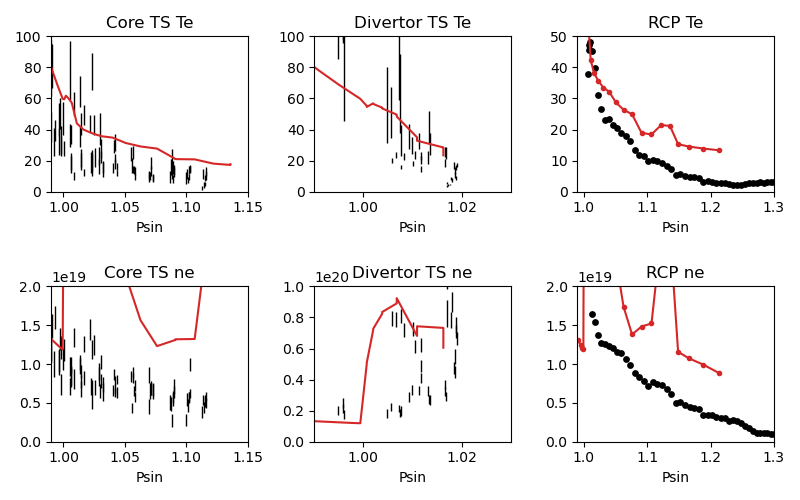
It is clear we still have some work to do! OEDGE (more specifically, OSM-EIRENE) generally overshoots both the experimental \(n_e\) and \(T_e\) data.
Obtaining agreement with experimental data - SOL 22
We have been calling the plasma solver within OEDGE OSM-EIRENE, but if you are using the code it will be useful to know this is referred to as “SOL 22” within the code. SOL 22 is a 1D fluid solver that solves the 1D fluid equation “from the targets up”. By successively solving the 1D fluid equation for each flux tube, or ring, a 2D plasma background is constructed. The solutions from one ring do not influence any others, and since we are only solving the 1D fluid equations anomalous transport coefficients (\(D_r\) and \(\chi_r\)) are not needed. This is a big strength of the 1D fluid approach. SOL 22 actually solves the 1D fluid equation twice for each ring, once for each half of the flux tube where it uses the respective target data from that half to generate the solution. The two solutions by default meet halfway along the flux tube, so there is often a mismatch in the two solutions there. This is not as big a deal as it seems. SOL 22 contains a number of options to control its behavior. These options represent experimental unknowns, either due to lack/error of measurement or simply physics that are not well-understood yet. Our input file uses all defaults, which results in a barebones SOL 22 simulation. We can do better.
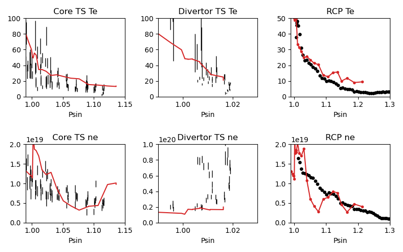
First, let us tell SOL 22 to iterate with the Monte Carlo neutral code EIRENE (P36 = 1). Let’s run EIRENE for 60 seconds (020 = 60) to reduce some of the noise inherent to Monte Carlo simulations. By default SOL 22 uses a set of simple analytic prescriptions for particle sources for the first iteration, and then uses EIRENE for further iterations. We also will turn off momentum losses (267 = 0) for now since they are on by default. Momentum losses within a flux tube can increase the density further upstream and the fact that we are overshooting the experimental density suggests we may have too strong of momentum losses near the target within our simulation. We add the following lines at the bottom of our input file:
$
$ Plasma background options - SOL 22
$
'*P36  Calculate SOL iteratively? 0-No 1-Yes              '  1
'*020  EIRENE run time (CPU seconds)                      '  60
'*267  Switch: Momentum loss    0-Off 1-On                '  0
Our match to experimental data is shown below.
This is better, but there is still some work to be done.
Next we will demonstrate how to modify the target conditions within the input file. We are able to scale the target data by user-defined constants with input options Q33 and Q35. You may have noticed that the match to the \(T_e\) data could be improved across the board were the target temperature decreased some. We can do this by adding the following options to our input file:
'*Q33  Inner Target Data Multipliers (Te, Ti, ne)         '  0.75 0.75 1.00
'*Q35  Inner Target Data Multipliers (Te, Ti, ne)         '  0.75 0.75 1.00
You may add these anywhere, but it is a good to put them near the target data that was input with options Q34 and Q36. Historically, Langmuir probes tend to measure higher \(T_e\) values relative to toher diagnostics, sometimes as much as double. It is therefore fine to decrease target temperatures if it helps the simulation agree with experimental data. The agreement improves, but density still leaves much to be desired.
We can investigate part of the problem by opening the .dat file and searching for “ERROR CORRECTION”.
LISTING OF ERROR CORRECTION LEVELS:
10 - TURN OFF EQUIPARTITION IF IT IS ON
 9 - REPLACE DENSITY GRADIENT DEPENDENT CROSS-FIELD TERM WITH UNIFORM
 8 - NO HEATING BY PINQI IS ALLOWED.
 7 - REPLACE WHOLE RING UNIFORM POWER WITH HALF RING UNIFORM.
 6 - HALF RING UNIFORM POWER AND HALF RING UNIFORM PARTICLES
 5 - HALF RING UNIFORM PARTICLES AND POWER IN AT TOP
 4 - 1/2 M V^3 CONVECTIVE TERM TURNED OFF
 3 - ALL ADDITIONAL POWER TERMS TURNED OFF
 2 - ALL CONVECTIVE TERMS TURNED OFF
 1 - CONDUCTION ONLY - ANALYTIC IONIZATION ONLY.

         ERROR SOLVER HAD A PROBLEM WITH THESE RINGS:
    RING        CODE   DESCRIPTION       POSITION     ERROR OPTION
      18 OUTER:   5   Excessive  T Drop      23.6883         5.0
      19 OUTER:   5   Excessive  T Drop      23.1212         5.0
      20 OUTER:   5   Excessive  T Drop      18.4019         6.0
      21 OUTER:   5   Excessive  T Drop      12.4305         5.0
      22 OUTER:   5   Excessive  T Drop      14.0135         5.0
      23 OUTER:   5   Excessive  T Drop      10.7760         6.0
      28 OUTER:   5   Excessive  T Drop      8.70605         6.0
      29 OUTER:   5   Excessive  T Drop      6.69045         6.0
      40 OUTER:   5   Excessive  T Drop      9.91743         6.0
      45 OUTER:   5   Excessive  T Drop      8.21199         6.0
      61 OUTER:   5   Excessive  T Drop      2.28877         6.0
      63 OUTER:   5   Excessive  T Drop      2.12353         6.0
      65 INNER:   5   Excessive  T Drop      7.09524         5.0
      66 INNER:   5   Excessive  T Drop      6.31839         5.0
      67 INNER:   5   Excessive  T Drop      6.62027         5.0
      68 INNER:   5   Excessive  T Drop      6.33202         5.0
      68 OUTER:   5   Excessive  T Drop      7.10495         5.0
      69 INNER:   5   Excessive  T Drop      5.84004         5.0
      70 INNER:   5   Excessive  T Drop      5.69753         5.0
      70 OUTER:   5   Excessive  T Drop      5.22396         6.0
      71 INNER:   5   Excessive  T Drop      5.15255         5.0
      71 OUTER:   5   Excessive  T Drop      6.24107         5.0
      72 INNER:   5   Excessive  T Drop      4.87548         5.0
      72 OUTER:   5   Excessive  T Drop      5.72123         5.0
     111 OUTER:   5   Excessive  T Drop      6.39845         6.0
This human-readable output file tells us that there are many SOL rings in which the error solver is kicking in. The error solver works by systematically turning off options within SOL 22 to simplify the problem down to one that does not throw errors in the solver. Error correction on a few rings is fine, but when many rings are encountering errors it is a good idea to simplify SOL 22 by turning off some of the extra options that are on by default. Two of these are the convection terms, which can sometimes destabilize the solver. We turn them off with the input options 254 and 255:
'*254  Switch: 5/2 nv * kT    : 0-Off 1-On                '  0
'*255  Switch: 1/2 m v^3 * n  : 0-Off 1-On                '  0
Turning these terms off improves agreement and allows the solver to run without error correction on nearly all the rings. The temperature agreement is decent, and density undershoots the experimental data across the board.
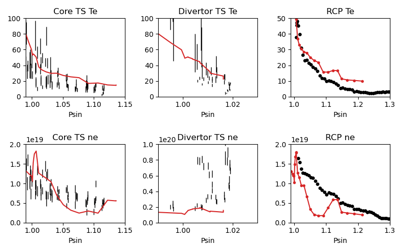
At this point in the process it is desirable that the density undershoots the experimental data because we can manually assign momentum losses to increase the density upstream of the targets (decreasing the density upstream does not have as convienent a “tool”). In the next section we take a relatively straightforward approach by manually assigning momentum loss “friction fractions” \(F_{fric}\) on each individual flux tube. See the documentation for 267 for a definition of \(F_{fric}\). For a grid such as ours with many rings in the SOL, this can be a time-consuming process but it generally is not too complicated. To save time, we will outline a semi-empirical method that can be used to automatically assign \(F_{fric}\) along each flux tube. The time saved by this approach comes at the cost of a little extra complication.
Assigning flux tube momentum losses (advanced)
The outline of this method is to perform a scan in \(F_{fric}\) to build a mapping between \(F_{fric}\) and upstream density for our simulation. We then determine the precise value for the \(F_{fric}\) needed to force agreement with experimental data. We will use the RCP data as our experimental constraint, this should leave us close enough to the Thomson data.
Begin by turning momentum loss back on with an expoentially decaying away from the target momentum source (267 = 2, consult the documentation for details). We will assign \(F_{fric}\) for the entire SOL with 242, where lower values correspond to larger amounts of momentum loss. Our SOL 22 options now look as such:
$
$ Plasma background options - SOL 22
$
'*P36  Calculate SOL iteratively? 0-No 1-Yes              '  1
'*267  Switch: Momentum loss    0-Off 1-On                '  2
'*242  Friction factor for Momentum loss formula          '  0.05
Save this file as d3d-167196-osm-v1-mom1.d6i to designate it as part of the \(F_{fric}\) scan. Change \(F_{fric}\) to 0.10 and save the file as d3d-167196-osm-v1-mom2.d6i. Continue in steps of 0.05 until you reach \(F_{fric}\) = 0.95 for a total of 19 different -momX files. Run every background with the same run command as before taking care to change the input file name for each command. This could easily be automated. If you are motivated enough to do this email Shawn and I’ll add it to the guide!
Note
Why are we assigning momentum losses? Aren’t those included in EIRENE?
Sort of. OEDGE is coupled to EIRENE07, as in a version from 2007. This version had questionable output with momentum losses turned on. It is possible that newer versions of EIRENE have resolved this issue, but EIRENE is a notoriously difficult code to understand and run, let alone to couple with another code. Future upgrades to OEDGE will certainly include coupling to a newer version of EIRENE, but for now the above workflow is good enough for obtaining experimentally constrained background plasmas.
With those runs in hand, we now need to write a script that can do all the interpolating necessary to answer the question, “What value of \(F_{fric}\) is needed for each ring to match the RCP \(n_e\) data?” An example script performing this task is shown below:
import oedge_plots
import numpy as np
import pandas as pd
from scipy.interpolate import interp1d

# Load the RCP data. Data has already been shifted inward by 1.5 cm due to EFIT uncertainties. Removing a couple
# bad data points.
rcp_path = "/Users/zamperini/Documents/d3d_work/divimp_files/oedge_tutorial/rcp_156195_2.csv"
rcp = pd.read_csv(rcp_path).iloc[:-4]

# Load OEDGE runs from F_fric scan, pull profile of ne at the RCP location, store in dictionary.
op_root = "/Users/zamperini/Documents/d3d_work/divimp_files/oedge_tutorial/"
ne_profs = {}
frics = np.arange(0.05, 1.00, 0.05)
for i in range(1, 20):
    op_path = "{}d3d-167196-osm-v1-mom{}.nc".format(op_root, i)
    op = oedge_plots.OedgePlots(op_path)
    ne_profs[frics[i-1]] = op.along_line(2.18, 2.30, -0.188, -0.188, "KNBS", "psin")

# For each ring, create an interpolation function of F_fric vs ne@RCP if possible.
f_f = {}
for ir in range(0, op.nrs):
    ne_at_rcp = []
    for fric in frics:

        # Mask for this ring. ir+1 is because OEDGE rings are 1-indexed, python is 0-indexed
        mask = np.array(ne_profs[fric]["ring"]) == ir+1

        # This shouldn't happen, but I (Shawn) haven't figured it out yet. It seems to not matter too much.
        if mask.sum() > 1:
            print("Warning! More than one value for ring {}".format(ir+1))
        if mask.sum() == 1:
            ne_at_rcp.append(float(np.array(ne_profs[fric]["KNBS"])[mask]))

    if len(ne_at_rcp) == 0:
        continue
    else:

        # Create interpolation function for F_fric(ne) so we can see what F_fric is needed for a desired ne value at
        # the location of the RCP.
        f_f[ir+1] = interp1d(ne_at_rcp, frics)

# For each ring with an interpolation function of F_fric(ne@RCP) find out what F_fric is needed to reproduce
# the RCP measurements. To do this we need an interpolation function of RCP_ne(psin).
f_rcp_ne = interp1d(rcp["psin"], rcp["Ne(E18 m-3)"] * 1e18)
fric_needed = {}
for ir in f_f.keys():

    # Get the ring's psin value so we can plug it into f_rcp_ne and get the desired density from OEDGE at the
    # RCP location.
    ring_psin = op.nc["PSIFL"][ir-1][0]  # 1-indexed to 0-indexed
    try:
        rcp_ne = f_rcp_ne(ring_psin)
        fric_needed[ir] = f_f[ir](rcp_ne)
    except ValueError:
        print("Ring {}: Outside of RCP data range - no value for F_fric given".format(ir))

# Now print out the data in a format that can be copy/pasted into input option *282.
print("'+242  Friction factor for momentum loss formula          '  1.0        # Default behavior is no momentum losses")
print("'*282  Momentum loss - ring specification                 '")
print("' ' '  Momentum loss - ring specification (dummy line)    '")
print("'  Ring   Ffric1     L1  Ffric2      L2    Number of rows:'  {}          # Only these rings have momentum losses".format(len(fric_needed)))
for ring, fric in fric_needed.items():
    print("     {}     {:.2f}    0.1    {:.2f}     0.1                   ".format(ring, fric, fric))
Running the script will output the following, which can be directly copy/pasted at the bottom of the input file:
'*242  Friction factor for momentum loss formula          '  1.0        # Default behavior is no momentum losses
'*282  Momentum loss - ring specification                 '
' ' '  Momentum loss - ring specification (dummy line)    '
'  Ring   Ffric1     L1  Ffric2      L2    Number of rows:'  14          # Only these rings have momentum losses
     22     0.78    0.1    0.78     0.1
     23     0.63    0.1    0.63     0.1
     24     0.40    0.1    0.40     0.1
     25     0.30    0.1    0.30     0.1
     26     0.24    0.1    0.24     0.1
     27     0.24    0.1    0.24     0.1
     28     0.68    0.1    0.68     0.1
     29     0.81    0.1    0.81     0.1
     65     0.90    0.1    0.90     0.1
     66     0.54    0.1    0.54     0.1
     67     0.64    0.1    0.64     0.1
     68     0.65    0.1    0.65     0.1
     69     0.77    0.1    0.77     0.1
     70     0.86    0.1    0.86     0.1
This contains input for two different options. Setting 242 = 1.0 sets the default value for \(F_{fric}\) equal to 1.0, which when looking at the equation in the documentation translates to no momentum losses on the rings. We then specify \(F_{fric}\) for individual rings with 282. This also includes values for the length of momentum loss region (we could set the default value with 243), which we keep at the default value of 0.1 (10% of the length of the field line). Note that the syntax for this type of input option requires a dummy line. Input options that begin with a * and take in a row of values require a dummy line, that’s just the way things are so we accept that and move on with our lives.
When we run our input file with the new momentum loss options the agreement with experimental data is improved.
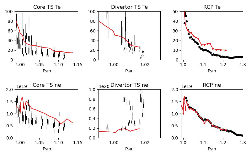
This is pretty decent agreement with the RCP! There is still some suspicious behavior near the separatrix though. This is because we only entered additional momentum losses for flux rings that overlapped with RCP data. The rings between the separatrix ring (16) and the first momentum loss ring above (22) are using default values so we should address that. Improving this is just good old fashioned trial and error. Add lines for the missing rings in the input file, and mess around with Ffric until you see decent agreement. An acceptable set of values is:
'*282  Momentum loss - ring specification                 '
' ' '  Momentum loss - ring specification (dummy line)    '
'  Ring   Ffric1     L1  Ffric2      L2    Number of rows:'  20          # Only these rings have momentum losses
     16     0.56    0.1    0.56     0.1
     17     0.85    0.1    0.85     0.1
     18     0.95    0.1    0.95     0.1
     19     1.00    0.1    1.00     0.1
     20     0.72    0.1    0.72     0.1
     21     0.72    0.1    0.72     0.1
     22     0.76    0.1    0.76     0.1
     23     0.79    0.1    0.79     0.1
     24     0.57    0.1    0.57     0.1
     25     0.41    0.1    0.41     0.1
     26     0.32    0.1    0.32     0.1
     27     0.29    0.1    0.29     0.1
     28     0.38    0.1    0.38     0.1
     29     0.41    0.1    0.41     0.1
     65     0.78    0.1    0.78     0.1
     66     0.93    0.1    0.93     0.1
     67     0.53    0.1    0.53     0.1
     68     0.55    0.1    0.55     0.1
     69     0.65    0.1    0.65     0.1
     70     0.65    0.1    0.65     0.1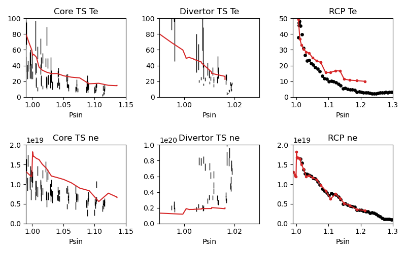
Note
I am noticing a sharp change in values across the separatrix, should I be worried?
It is generally impossible to get a smooth variation across the separatrix due to the relatively simple core plasma prescription in OEDGE. For our scenario, we have constant conditions along the core rings. Therefore a seamless transition in plasma density across the separatrix at the outboard midplane would mean there is a discontinuity everywhere else. This is because the plasma along the SOL field lines changes according to the 1D fluid equations. The best we can do is to keep the discontinuity to a minimum, either by continually finetuning our solution or shifting the experimental data within its error. We don’t focus too much on this here, but it is always an option.
At this point we may consider our background plasma sufficiently constrained. It is clearly not perfect: the temperature still overshoots the RCP and Thomson scattering data some, the density doesn’t agree as well with Thomson scattering, and the divertor Thomson scattering seems to indicate higher densitiles than what OEDGE is producing. Also when we input the target data in Q34 the rings without data are assigned “the values for the next inward - i.e. lower numbered ring are used”, see documentation. It would be better to have values for each ring, but this is a large grid and would take time. It may be possible to improve agreement by continuing to mess with the SOL 22 options or manipulating the experimental data further, but this can also be time consuming. If better agreement is important to your study, then take the time to try and obtain it! You can download the final input file used to generate the background here.
For the purposes of this guide we will consider ourselves finished with the background plasma and will move on to simulating the transport of tungsten in this background plasma.