Performing Impurity Transport Simulation with DIVIMP
Note
This section assumes you completed the previous section on Generating an OSM-EIRENE Plasma Background as that background plasma is used for the DIVIMP simulations here.
DIVIMP is the Monte Carlo impurity transport code within OEDGE. It handles the sourcing of impurities from target elements, the transport of those impurity ions throughout the plasma, and performs the necessary statistics to calculate things like impurity density or radiation. It operates under the trace impurity approximation, which assumes that the impurity density is low enough that is has no effect on the background (deuterium) plasma quantities. Impurity transport experiments are sometimes designed with this in mind, making DIVIMP an ideal tool for investigating SOL impurity transport.
For this guide, we will simulate tungsten (W) transport in DIII-D discharge #167196. This discharge was part of the DIII-D Metal Rings Campaign where two toroidal rings of W tiles were installed in the lower outer divertor, one on the shelf and the other on the floor tiles. A layout for the discharge we are modeling is shown below.
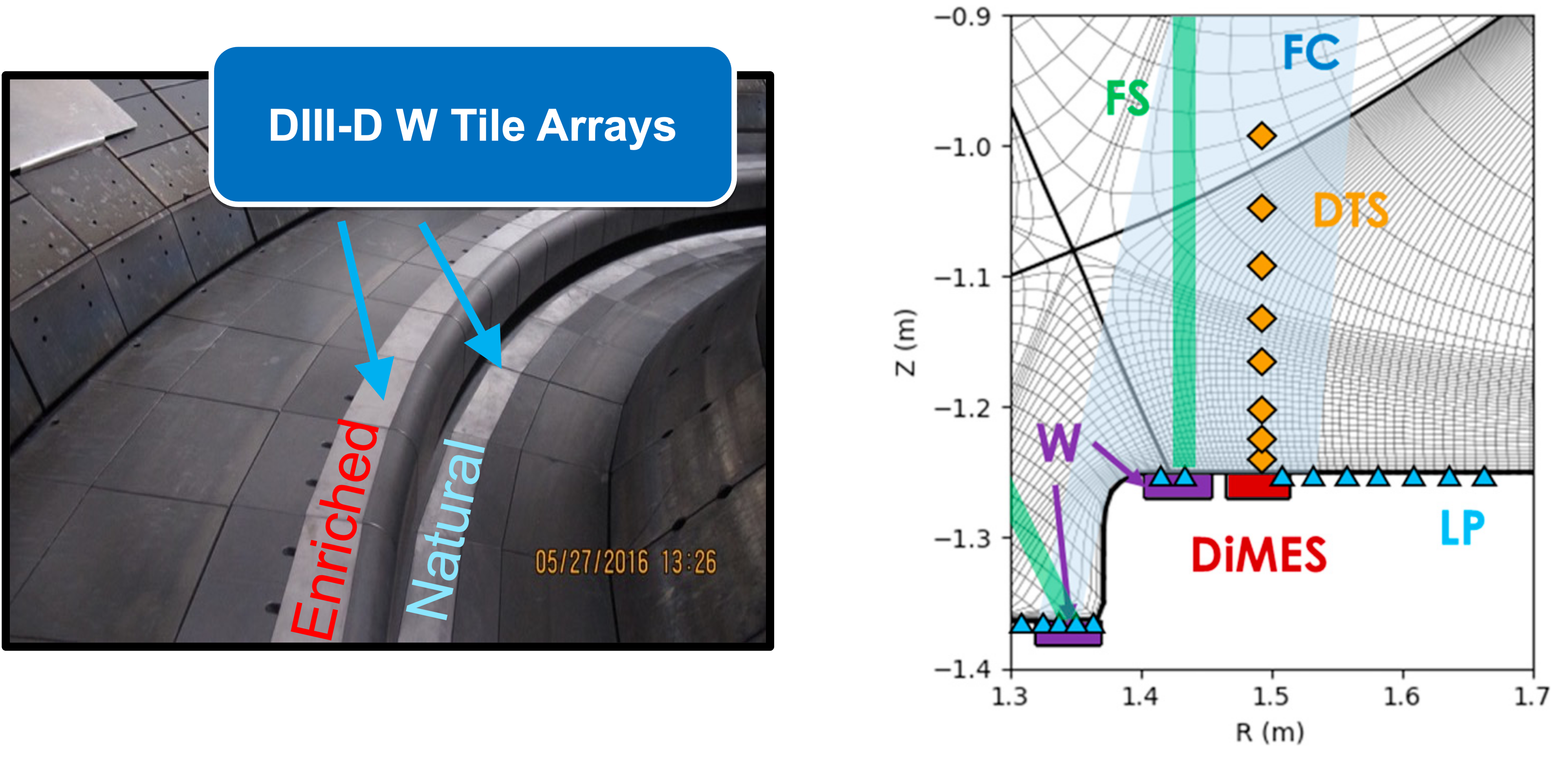
No erosion was observed from the floor ring since it was in the PFZ, therefore from here on out we will only focus on the shelf ring, where the strike point was positioned. Let us begin by setting up the input file to track W. We have two options here. We can either modify our background plasma input file from the previous section of this guide to follow W impurities after generating the background, or we can use a set of options that allow us to pass in a previously generated background plasma. We opt for the latter in order to not waste computational resources. We open a blank document and add the following lines, similar to when we setup the input file for the plasma background in the previous section:
$
$ Required to indicate extended grid generated by Fuse.
$
'{GRID FILE}     File name of the fluid grid to be loaded '  'fort.4'
'{GRID FORMAT}                                            '  2
'{EXIT}'
$
$ Options related to reading in plasma background
$
'*P01  SOL option     98 = Read OEDGE file                '  98
'*P02  Core Option    -1 = Do nothing (read from file)    ' -1
'*P03  Plasma decay   98 = Read OEDGE file                '  98
'*Q01  TeB Gradient   98 = Read OEDGE file                '  98
'*Q02  TiB Gradient   98 = Read OEDGE file                '  98
Next we need to add some options specifying that W we are simulating W and some of the transport related input options.
$
$ DIVIMP - Options for W transport
$
'*S04  Mass of impurity ions (amu)                        '  183.84
'*S05  Atomic number of impurity ions                     '  74
'*I15  Maximum ionization state                           '  74
'*D04  USERID for ADAS Z data (*=use central database)    '  '*'         # ADAS is configured on iris, you don't need to worry about
'*D05  Year for ADAS Z data                               '  50          # W = 50 (C = 96 just FYI)
'*T14  SOL diffusion coefficient (m2/s)                   '  0.3         # 0.3 m2/s is a good starting point for the SOL
'*S11  Number of impurity ions to be followed             '  5000        # 1000 is good for rapid testing, then crank this up for publication quality
'*G14  Core mirror ring                                   '  8           # Not too interested in core transport, this cuts down on simulation time
'*S14  Quantum iteration time for ions (s)                '  1.0e-7      # Default is 1e-8 s, but 1e-7 is fine and cuts down on simulation time
Now we need to specify how the W is being sourced into the simulation. What follows are a set of options to study W transport assuming all the W is sputtered by a flux C2+ atoms that is 2% of the background deuterium plasma flux to the target.
$
$ DIVIMP - Launch W from shelf ring due to 2% C2+ impact
$
'*D22 ' 'Yield Modifiers for neutrals                     '
' ' '    Yield Modifiers for neutrals (dummy line)        '
'  ID1  ID2    Mpt   Mst   Mct   Mpw   Mcw  Refl     Rows:'  3
     1  158    0.0   0.0   0.0   0.0   0.0   1.0
   159  164    1.0   1.0   1.0   1.0   1.0   1.0    # Shelf ring, R = [1.404, 1.454]
   165  213    0.0   0.0   0.0   0.0   0.0   1.0
'*N08  Sputter option  1 = Sputtering by specified ion    '  1
'*D07  Sputter data option (5 used for C-->W)             '  5
'*D18  Bombarding ion charge state                        '  2
'*D19  Bombarding ion type (5=Carbon)                     '  5
'*D40  Bombarding ion flux fraction                       '  0.02
Input option D22 may be a little confusing if you are seeing it for the first time. The documentation has the details, but all we are doing is assigning a “yield modifier” of 1.0 to all the wall segment that span the W ring, and then 0.0 to every other segment. In this way we simulate W sourcing from just the W ring. You can find the wall indexes by looking at the “NEUTRAL WALL ELEMENT LISTING” table within the .dat file from a previous simulation that uses our grid, such at the background simulation .dat file. There are various sputtering options that can be specified via N08, we chose the one that allows us to specify W is sputtered by C2+ ions (D18, D19 and D40).
With the above input options saved in a file called d3d-167196-divimp-csput-v1.d6i, we may run this case on iris with the following run command:
./rundiv.sh d3d-167196-divimp-csput-v1 d3d_bkg grid_d3d_167196_3000_v1 none none d3d-167196-osm-v1
We have passed in the background plasma d3d-167196-osm-v1. It is assumed that this was a previous OEDGE case and thus the resulting output files are stored in your results directory. This run took about 25 minutes on iris.
You can use the plotting GUI to make some simple plots of the impurity density, but the scripting mode of OedgePlots contains signficiantly more flexibility in the type of plots you can make. We show some examples of this with the following script.
import oedge_plots
import matplotlib.pyplot as plt
import numpy as np


# Load run into OedgePlots object.
ncpath = "/Users/zamperini/Documents/d3d_work/divimp_files/oedge_tutorial/d3d-167196-divimp-csput-v1.nc"
op = oedge_plots.OedgePlots(ncpath)

# 2D plot of the W density (all charge states).  DDLIMS is the name of impurity density array in netCDF file. It
# must be scaled by op.absfac to go from normalized to physical units.
op.plot_contour_polygon("DDLIMS", charge="all", normtype="log", cmap="inferno", lut=7, vmin=1e9, vmax=5e15,
                        scaling=op.absfac, cbar_label="W Density (m-3)")

# 2D plot of just the W15+ density.
op.plot_contour_polygon("DDLIMS", charge=5, normtype="log", cmap="inferno", lut=7, vmin=1e9, vmax=5e15,
                        scaling=op.absfac, cbar_label="W5+ Density (m-3)")

# 2D plot of the W concentration. We make use of the own_data parameter to pass in manipulated data. We can mask the
# data so it doesn't plot anything where it equals zero.
wdens = op.read_data_2d("DDLIMS", charge="all", scaling=op.absfac)
ne = op.read_data_2d("KNBS")
wconc = np.ma.masked_where(wdens==0, wdens / ne)
op.plot_contour_polygon(own_data=wconc, normtype="log", lut=5, cbar_label="W Concentration", cmap="cool",
                        vmin=1e-8, vmax=1e-3)

# Plot of the W density along the separatrix ring.
s, nw = op.along_ring(op.irsep, "DDLIMS", charge="all", plot_it=False, scaling=op.absfac)
fig, ax = plt.subplots(figsize=(5, 4))
ax.plot(s, nw, color="k", lw=3)
ax.plot(s, nw, color="tab:red", lw=2)
ax.set_yscale("log")
ax.set_xlabel("Distance from inner target (m)", fontsize=12)
ax.set_ylabel("W Density (m-3)", fontsize=12)
ax.grid(alpha=0.3, which="both")
fig.tight_layout()
fig.show()

# Plot of the W density at the outboard midplane. Zeros are masked.
w_dict = op.along_line(2.18, 2.30, op.z0, op.z0, "DDLIMS", charge="all", scaling=op.absfac)
mask = np.array(w_dict["DDLIMS"]) > 0
x = np.array(w_dict["psin"])[mask]
y = np.array(w_dict["DDLIMS"])[mask]
fig, ax = plt.subplots(figsize=(5, 4))
ax.plot(x, y, color="k", lw=3)
ax.plot(x, y, color="tab:red", lw=2)
ax.set_yscale("log")
ax.set_xlabel("Psin", fontsize=12)
ax.set_ylabel("W Density (m-3)", fontsize=12)
ax.grid(alpha=0.3, which="both")
fig.tight_layout()
fig.show()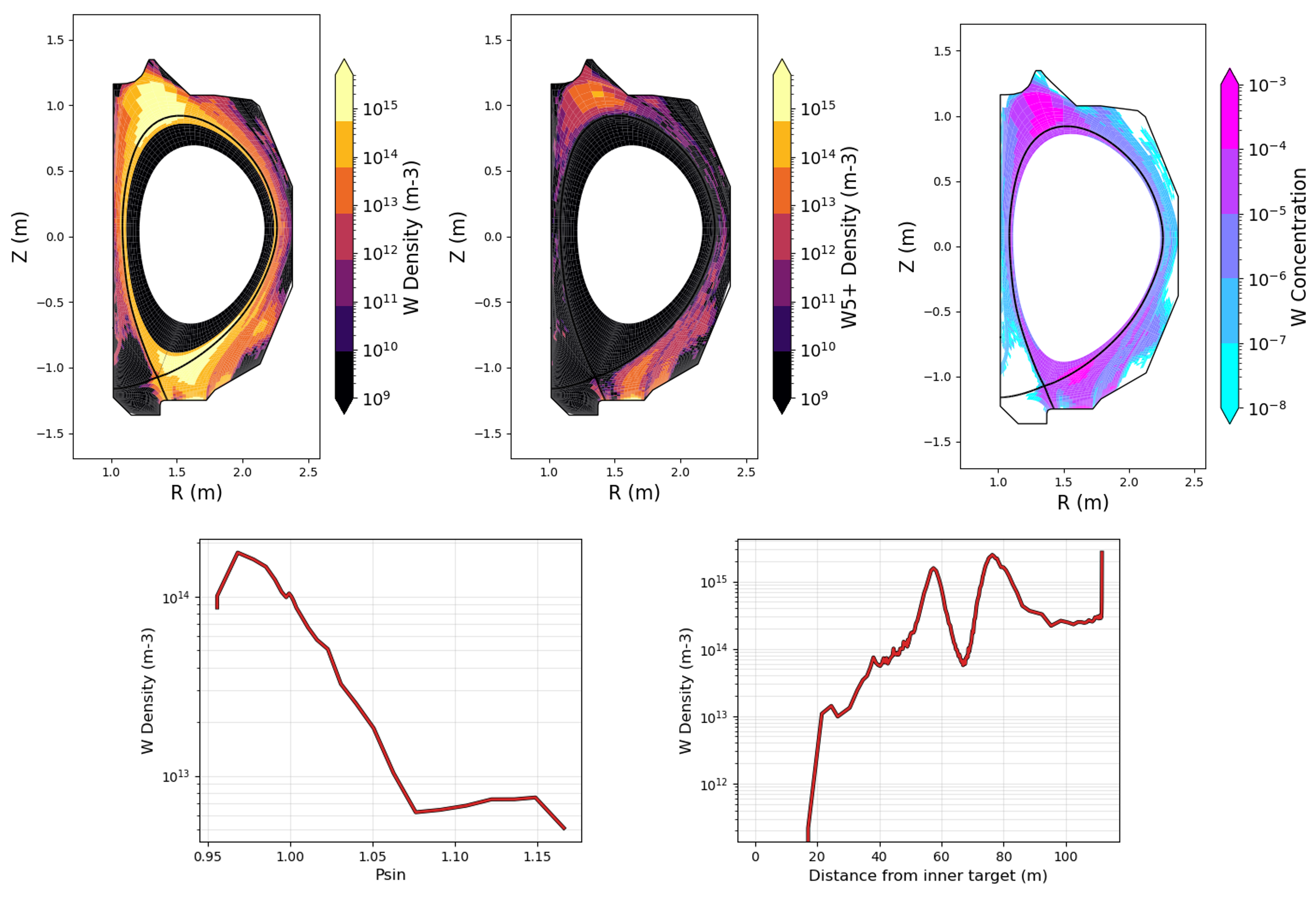
We notice that W accumulates about halfway between the targets, creating a zone of elevated density/concentration near the top of the plasma. This is primarily due to the main ion temperature gradient and has been studied with DIVIMP extensively (see Publications).
ExB drifts are turned off by default. We can turn them on with the following input options:
'*T37  ExB radial drift    0=Off 1=On                     '  1
'*T38  ExB poloidal drift  0=Off 1=On                     '  1
'*T39  ExB drift scale factor  + = LSN, forward BT        '  1.0
T39 scales the strengths of the drifts, values less than one weaken it and greater than 1 strengthen it. A previous study found 0.6 reproduced measurements on DiMES, but please do mess around with it.
You can download the final version of the input file for this section here.
This concludes the OEDGE Beginner’s Guide. In summary, we:
Created our workspace on iris and setup our local computer for data and simulation analysis
Created grids using DG-Carre and the extended grid generator Fuse
We used the extended grid to create a plasma background using the OSM-EIRENE (SOL 22) input options within OEDGE
We simulated W sputtering from W rings inside DIII-D due to 2% C2+ impact
This is clearly a very specific application of OEDGE, and your cases will naturally be different and want to investigate different output. Fortunately, the process outlined here can be generalized to any device. The unknowns mainly involves how to access daat from the device and the general data transfer protocol. A natural question at this point is how do I find out what other input options are available to me?
What next?
There are many other input options you can use to generate plasma backgrounds and simulate impurity transport. The page Input Options contains many of the input options, many of which still need to be detailed. If this isn’t enough, essentially all the relevant input options and their defaults can be found by looking in the oedge/master/div6/src/f90/mod_unstructured_input.f90 and oedge/master/comsrc/f90/mod_sol22_input.f90 source files. Of course, we hope to eventually have all this information on this website, but these files are where that information comes from. Finally, OEDGE has a community of users and communication is encouraged! If interested, reach out to Shawn Zamperini (zamperinis@fusion.gat.com) and ask about being added to the Discord server.