Creating a Plasma Grid
OEDGE simulations of the SOL require a field-aligned mesh with which to perform their calculations on. An excellent video demonstrating how the complex curviliner grids used in SOL codes are converted to a simple 2D Cartesian grid can be seen by following this link.
There are two options for generating a grid for OEDGE:
DG-Carre: This is the most common option. It is the same grid generator used by the 2D SOL fluid code SOLPS-ITER, and so documentation on how to use it is available.
FUSE: Some time ago a grid generator was built in the IDL programming language to deal with the limited radial extent of DG-Carre grids. It is largely a black box in that it either works or it doesn’t, and the grids are specific to OEDGE only.
Instructions on generating a grid via both methods will be included here.
DG-Carre Grid
DG is a GUI used for manipulating and setting up grid making, while Carre is the software that actually makes the grid. Both are very old. To use DG-Carre, we will be setting up your workspace within the SOLPS-ITER directory. This is as standardized a way as there can be in this field, so we will stick to convention.
First, create your solps-iter directory and copy over the needed files:
cd /fusion/projects/solps-results
mkdir [username]
cd [username]
mkdir runs post dg-carre
cd dg-carre
cp –r /fusion/projects/solps-results/share/dg-carre_share/* .
Next we want to configure your .bashrc file to include all the needed aliases. Your .bashrc file is in your home directory on iris (geany ~/.bashrc).
export OBJECTCODE='linux.pgf90'
export TOKAMAK='D3D'
alias solpsiter_public='pushd /fusion/projects/codes/solps/SOLPS-ITER/public_code/solps-iter_release_sept2019;source setup.ksh;popd'
export SOLPSTOP="/fusion/projects/codes/solps/SOLPS-ITER/public_code/solps-iter_release_sept2019"
export DGHOME="/fusion/projects/solps-results/[username]/dg-carre"
alias dghome='cd /fusion/projects/solps-results/[username]/dg-carre'
alias dg='/fusion/projects/solps-results/[username]/dg-carre/DivGeo/dg/linux.ifort64/dg'
alias e2d='/fusion/projects/solps-results/[username]/dg-carre/DG/equtrn/e2d'
alias dg2dg='/fusion/projects/solps-results/[username]/dg-carre/DG/equtrn/linux.pgf90/dg2dg'
alias xmatlab='cd /fusion/projects/solps-results/[username]/post/scripts; matlab &'
Don’t forget to substitute your iris username in for [username]. Your .bashrc file is sourced every time you login, but for now since we’ve modified it we need to source it manually: source ~/.bashrc.
Now we want to to download an equilibrium (i.e., the “gfile”), convert it to a format for DG and then increase the resolution of it.
$ dghome
$ cd class
$ mkdir d3d_[username]
$ cd d3d_[username]
$ mkdir 167196_3500
$ cd 167196_3500
$ idl
$ writeg,167196,3500
$ exit
$ e2d g167196.03500 output.eq
$ dg2dg output.eq outputx2.eq
$ dg2dg outputx2.eq outputx4.eq
$ dg2dg outputx4.eq outputx8.eq
Before we open up DG, we first will want to copy over an .ogr file, which is just a file of the R, Z coordinates of the most limiting surfaces of the DIII-D wall, into the current directory.
$ cp /fusion/projects/codes/oedge/zamperinis/data/d3d_wall_geometry_june2016.ogr .Note
This .ogr file is from June 2016, which is when shot #167196 ran. When doing your own discharge, you will need to use the corresponding wall coordinates as the DIII-D wall frequently changes. Ask around if anyone already has the file made, particularly the SOLPS-ITER people. If one cannot be found, you can extract the coordinates from the gfile. This is perhaps easiest by creating the gfile in the OMFIT EFIT module and copying over the coordinates. In the OMFIT tree, you find the R, Z coordinates at
OMFIT["EFIT"]["FILES"]["gEQDSK"]["RLIM"]and"ZLIM". Copy that data over into a text file in the same format as the .ogr file.
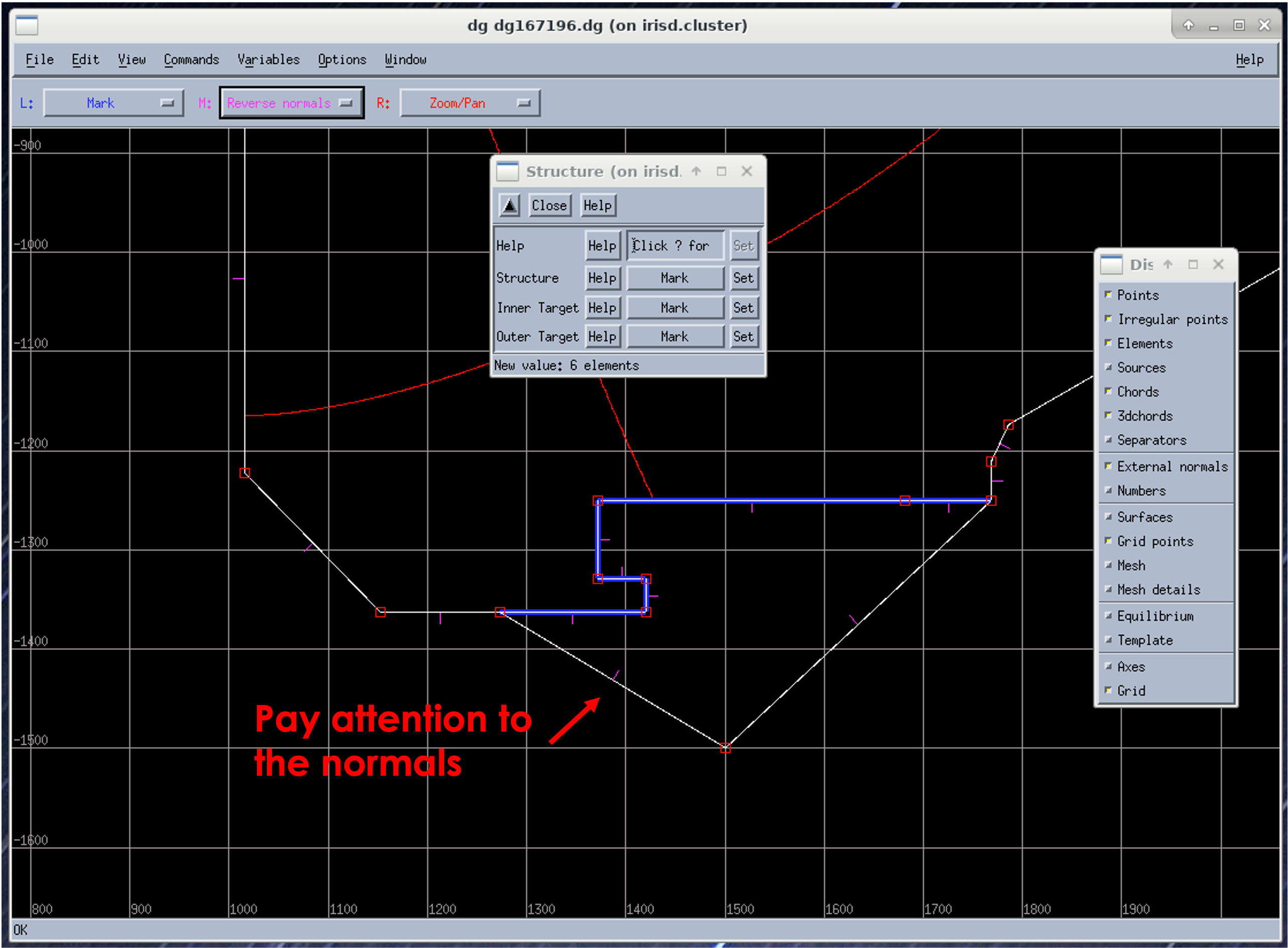
Now open up DG with dg &. First import the .ogr file: File > Import > Template. Use Ctrl+P to reset the view. Next, convert the template to elements via Commands > Convert > Template to elements. Your screen should look like something this:

Note we have changed the actions on each of the left (L), center (M) and right (R) mouse clicks. It is good practice to make the L and R actions something benign, like Mark and Zoom/Pan, to avoid accidentally performing an action you didn’t mean to. As we will learn, DG can be finnicky and so we must work slowly and diligently. With that said, save often! File > Save and then name your file something like dg167196.dg.
For our first action, we are changing M to “Reverse normals”. Hover over an element and click M to reverse the normal (the direction of the pink line). We need to reverse all the normals, and fortunately there is a shortcut. To perform an action on all elements, hold down shift when clicking the button, e.g., Shift+M. All the lines should now be pointing away from the plasma like in the image above.
Next, we import the equlibrium: File > Import > Equlibrium. Select the file outputx8.eq. Now import the topology: File > Import > Topology. The topology options are found in $DGHOME/DivGeo/dg/topologies. If this directory is blank, you may just have a file filter on. At the top bar make sure it ends with a * and not a filter such as *.dg (* is called a wildcard, meaning it will match anything). This discharge uses the SN topology, so select that one. The topology identifies the separatrix.
Once we’ve identified the separatrix, we no longer want the red/blue equlibrium on our display as it will quickly get crowded. Let’s get a pop-out of the display options as they are handy to have nearby. Click View > Display, and then drag your mouse on the top-most set of dashed lines. This will pop the Display options out to a separate window. Your screen should now look like the following:

Now we must define the target surfaces. These determine how wide your grid will go, at least up until it hits some other limiting surface that prevents the field line from connecting between both targets. Go to Variables > Structure. To set the elements for each target, Mark (we assigned this to L) each segment and then click the Set button in the Structure window. In the below, we have selected the following 3 elements for the inner target (I have turned on the “Points” Display option):

Note
Before marking and setting any elements, it is a good habit to always ensure that you have not accidentally marked any other objects. This can create headaches later on down the road. You can unmark all objects, if any are marked, with Ctrl+U.
For the outer target we set the following elements:

Before we do the same for Structure, there is one pecularity we must take care of first. DG-Carre requires that the targets be closed polygons. This means we need to create imaginary elements outside of the vessel that make each target a polygon. Whatever shape this polygon is does not matter, just that it needs to be there. To do this, go to Edit > Create > Point. For the outer target, create a point at 1500, -1600. We want to create elements connecting the end points of the outer target to this point (Tip: You can see the end points by Ctrl+U and then clicking Mark in the Structure window for the Outer Target). Set M to Connect Points. Click and drag between the two end points of the outer target. The surface normals must always be facing the inside of the polygon, so switch M to Reverse Normals and click the segments where the normal is facing the wrong way. Your outer target should now look like the following:
Repeat for the inner target by creating another point at 900, -1300 and connecting the points. Pay attention to the normals!

Now, to set the Structure elements mark ALL elements. Shift+L (assuming L=Mark) allows you to drag a box over everything. Then UNMARK the indicated three elements that separate the targets from the rest of the structure:

If there were more than just a single element separating the inner and outer targets in the PFZ, you would select just the first elements outside out each defined target, like we are doing for the SOL side of the targets.
Each target needs a SOL and a PFZ edge element designated. Navigate to Variables > Target Specification > #1. Which target corresponds to which target number depends on the configuration:
#1: inner target (LSN), outer target (USN), lower inner target (DN)
#2: outer target (LSN), inner target (USN), upper inner target (DN)
#3: upper outer target (DN)
#4: lower outer target (DN)
#167196 is LSN, so Target #1 is the inner target. Mark the furthest out element within the SOL (Ctrl+U first!) and click Set for SOL Edge. Likewise, pick the element furthest into the PFZ and click Set for PFR Edge. Repeat for Target #2 (the outer target). Now is a good reminder to save often if you haven’t been!

We are now ready to create flux surfaces. The first step is to create an innermost flux surface in the core to define the inner extent of the mesh. Set M to Add Surface, and then click somewhere in the core and release to create the inner surface. Then open Edit > Create > Surface(s).
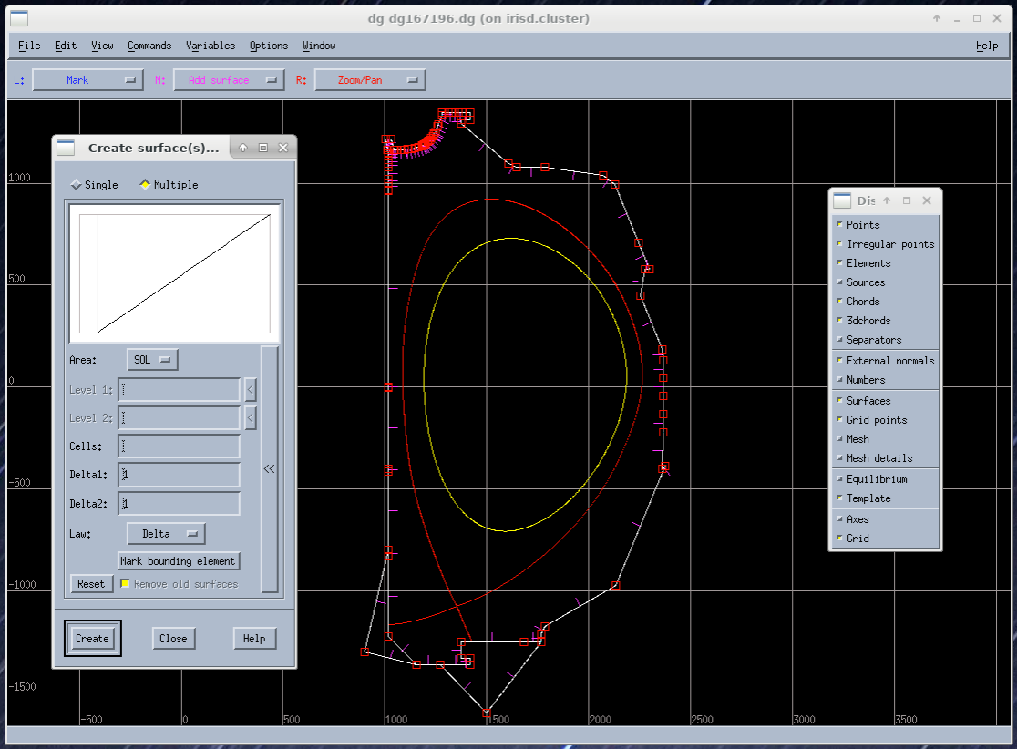
The Area variable defines the region within which flux surfaces are created. The Cells variable defines the number of flux surfaces for that region. The Delta1 variable defines the spacing between flux surfaces near the X-point. The Delta2 variable defines the spacing between flux surfaces at the other end. You can drag the line to get the desired spacing (see image). Follow the guidelines below when creating flux surfaces:
OEDGE can handle finer grid than SOLPS-ITER (for those who have already seen such grids), which generally stick to around 20-30 surfaces in each region. There is no hard and fast rule for OEDGE here, but 20 surfaces within the Core and PFZ and 50 within the SOL is a decent starting point.
Make sure that the number of flux surfaces is the same within the core and the PFZ.
Make flux surface spacing small near the X-point and large away from the X-point. The increase in flux surface spacing should be nonlinear.
Flux surface spacing should be the same across the X-point in all directions. Users should start with the PFR region and adjust spacing relative to the settings for the PFR region.

Next is to create grid points, which determine the poloidal resolution of the grid. Go to Edit > Create > Grid Point(s). The Zone variable defines the part of the separatrix along which grid points are created. The Cells variable defines the number of grid points for that zone. The Delta1 variable defines the spacing between grid points near the X-point. The Delta2 variable defines the spacing between grid points at the other end. Make sure that the Law variable is set to “Delta.” You can also drag the plot to get the desired grid spacing. Follow the guidelines below when creating grid points:
Keeping the total number of grid points (sum of the outer divertor, inner divertor and SOL) to around 200 is probably a good starting point.
Unlike flux surfaces, the number of grid points in each zone do not need to be the same. Make sure that there are a sufficient number of grid points in each divertor zone to yield a high resolution near the target surfaces.
Make grid point spacing smaller near the target (Delta2) and larger near the X-point (Delta1) for the divertor zones.
Make grid point spacing smaller on both ends for the SOL zone. An easy way to do this is to set Delta1=Delta2. Reduce the Delta value to reduce the grid point spacing near the X-point.
The grid point spacing should be roughly the same across the X-point in all directions. Below image shows acceptable spacing around the X-point - it doesn’t have to be exact.

Now we are just about ready to move onto Carre and to try and generate the actual grid. Before this, go to Commands > Check Variables. This should give a little message in the bottom left of the screen that says, “All variables have valid values”. Then click Commands > Rebuild Carre Objects. This has no output, we just trust it does whatever it does correctly. Then click File > Output and press OK.
Return to your terminal and change to your class directory: cd $DGHOME/class. Run the linking scripting, e.g., ./lns d3d_[username]/167196_3500/dg167196. Do not include .dg in the command. Then navigate to the Carre directory with cd $DGHOME/Carre and run Carre with ./carre -. As an example:
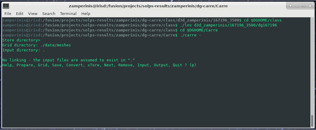
Carre is run in the following order: Prepare (P), Grid (g), Convert (c), Store (t) and Quit (q). If life was great, we would only need to run this once and we’d have everything we need. Unfortunately, Carre often generates a number of errors and it’s largely a black box on how it works (it doesn’t help that much of the code is documented in French). The values that work for this tutorial may not necesarilly be the ones that work for the grid you are constructing. Nonetheless, you will encounter this step every time, so it is worth learning how to get around. Some tips:
Often decreasing pasmin will solve some errors
Pay attention to what zone it has issues with, the error message tells you
Often just small changes are all that’s needed. So if the error says to change deltr1 and deltrn in zone 2, and you see that they are -4.8467E-4 and -4.213E-2, then try setting them to -0.00001 and -0.001, respectively (i.e., decrease them by a factor of 10).
Sometimes this just comes down to random, dumb luck. I’m sorry.
If you can get through the Grid step, the rest is just hitting Enter at each step until Carre finishes. Next we wish to load the generated grid into DG and inspect it. In DG go to File > Import > Mesh. The grid is stored at $DGHOME/Carre/data/meshes. If you’re lucky, you will have the following purple grid loaded into your session.

Congratulations! You’ve made your first grid. The file you need for OEDGE will be the one saved as $DGHOME/Carre/data/meshes/dg167196.v001.griddivimp, that is, the .griddivimp extension is saved in the format needed to be read by OEDGE. You can download the grid generated by this guide here.
Troubleshooting
I loaded my grid into DG, but some of the cells are pink. What does that mean? Your grid has issues with cells not being orthogonal. Go back into Carre and tweak some of the parameters to generate a new grid. Repeat until the loaded grid has no pink cells.
FUSE Grid
As an alternative to DG-Carre, OEDGE has support for an additional grid type generated by the scripts within the FUSE repository, collectively called GRID. These are sometimes just referred to as “extended grids” due to the fact GRID grids generally fill in more of the vessel. If one is particularly concerned with plasma far out in the SOL, they may want to consider making the grid with GRID instead of DG-Carre. GRID may also be a bit easier to use since it hides most of the grid making magic behind the scenes, but it is largely a black box as to how it works. In this section we detail how to download the required scripts on iris and how to make the grid.
A memo on GRID can be seen by clicking this link. We will repeat all the needed instructions for using GRID on this page, but the memo may be useful for anyone needing to run GRID on a machine other than iris.
Open up your .bashrc file and add the following lines at the bottom of it:
export FUSEHOME=/fusion/projects/codes/oedge/fuse
alias cdf='cd $FUSEHOME'
alias cdfo='cd $FUSEHOME/src/osm'
alias cdfe='cd $FUSEHOME/src/eirene07'
alias cdfi='cd $FUSEHOME/input'
alias cdfl='cd $FUSEHOME/idl'
alias cdfs='cd $FUSEHOME/shots'
alias cdfr='cd $FUSEHOME/results'
alias cdfc='cd $FUSEHOME/cases'
export PATH=$PATH:$FUSEHOME/scripts
Next open up your .cshrc file and add the following at the bottom of it:
setenv FUSEHOME "/fusion/projects/codes/oedge/fuse"
alias cdf  cd $FUSEHOME
alias cdfo cd $FUSEHOME/src/osm
alias cdfe cd $FUSEHOME/src/eirene07
alias cdfi cd $FUSEHOME/input
alias cdfl cd $FUSEHOME/idl
alias cdfs cd $FUSEHOME/shots
alias cdfr cd $FUSEHOME/results
alias cdfc cd $FUSEHOME/cases
setenv PATH $PATH":$FUSEHOME/scripts"
setenv IDL_STARTUP $HOME/idl_startup.pro
Then make sure to source the file after saving it with source ~/.bashrc (unclear if you actually need to source .cshrc, but you can do it by entering a C Shell with csh and then source ~/.cshrc. Exit csh and go back to bash with just bash). Now navigate to the fuse directory and create a directory where you will make the grid:
$ cdf
$ cd shots/d3d
$ mkdir [iris_username]_167196
$ cd [iris_username]_167196
Next we need to download the gfile into our folder. This can quickly be done with:
$ idl
> writeg,167196,3000
> exit
You may note that we are using a different time than in the DG-Carre section of the guide (3000 vs. 3500 ms). The reason is when making this tutorial there were issues encountered with 3500 that didn’t occur during 3000 ms. No idea why, but like we said, GRID is a black box so sometimes you just need to try different things.
Note
There is sometimes a compatability issue with the gfile and GRID if your save the gfile via python where there are not spaces before the minus signs in the gfile. To address it, we must open the gfile with
geany g167196.03000 &. Go to Search > Replace. Make sure “Use regular expressions” is checked. Copy the following regex into the “Search for:” box(?<=[0-9])-. Copy the following into the “Replace with:” box\ -(that is a space and then a minus sign). Then click the “In Document” button to add a space before every minus sign.
Now we run the following command to create the needed .equ files:
$ fuse -equ d3d [iris_username]_167196 g167196.03000 d3d_167196_3000
You will now see various .equ files within your directory (for those who have made a DG-Carre grid, these are the same .equ files, just likely a bit higher resolution). Now we need to copy over all the needed IDL scripts to run GRID. Run the following commands within the [iris_username]_167196 directory:
$ cp -r $FUSEHOME/idl .
$ mkdir idl/grid_data
Next run:
$ fuse -make grid-iris [iris_username]_167196
Open up the file idl/grid_input.pro within your [iris_username]_167196 directory. This is a confusing file, but we only need to change a small section of it. Scroll down to where it says 'd3d': BEGIN. This contains the limited amount of input options we control. First, let’s specify our wall file. Scroll down to where you see wall_file and change the entry to wall_file = 'vessel_wall_mod_omp_lot_uit.dat'. This is a modified wall file that has been optimized for the extended grid generator to allow grids that extend all the out to the outer wall. The other options determine the extent and resolution of the grid to generate. The entries in ctr_boundary set the bounds in psin space. The other entries determine the poloidal resolution of the grid (pol_res_min, pol_res_max) and the radial spacing of the rings in the core/PFZ (rad_res_core_min, rad_res_core_max) and the SOL (rad_res_sol_min, rad_res_sol_max). xpoint_zone defines a box [R1, R2, Z1, Z2] that contains the X-point. Sometimes you may need to restrict this to the X-point region if it is erroneously labeling other magnetic nulls as X-points. For this tutorial, set the following options, you can ignore all the other options:
user_step   = -0.0001D
user_finish = 0.1000D
option.ctr_boundary = [ -0.80D*user_finish  ; CORE PSIn boundary
                         1.80D*user_finish  ; SOL
                         1.20D*user_finish  ; SOL, LFS (unused here)
                         0.02D*user_finish  ; SOL, HFS (unused here)
                        -0.20D*user_finish  ; PFZ
                        -0.015D*user_finish] ; PFZ, SECONDARY (unused here)
option.pol_res_min = 0.0005D  ; sets the poloidal length of the cells at the target
option.pol_res_max = 0.0500D  ; sets the poloidal length of the cells upstream
option.rad_res_core_min = 0.0005D  ; radial size of the core ring closest to the separatrix
option.rad_res_core_max = 0.100D  ; radial size of the core rings far from the separatrix
option.rad_res_sol_min = 0.0005D   ; radial size of the core ring closest to the separatrix
option.rad_res_sol_max = 0.050D   ; radial size of the core rings far from the separatrix
xpoint_zone = [1.0,2.0,-1.2,1.2]
wall_file = 'vessel_wall_mod_omp_lot_uit.dat'
These settings have already been tinkered with to generate a substaintially extended grid. We will first run the preview option to get a sense of what region our grid may fill in.
$ fuse -make grid
$ fuse -grid-iris -preview d3d [iris_username]_167196 167196_3000.x16.equ test
You should get something like the following output:

This plot is telling us what the settings in the input file are telling GRID to do. The blue line is setting the radial extent of the generated grid in the SOL (if it can even be generated that far out without an error). Likewise for the red line in PFZ and yellow for the core. Run the same command but without -preview to generate the grid. This may take around 15-20 minutes.
$ fuse -grid-iris d3d [iris_username]_167196 167196_3000.x16.equ test
The grid is saved as “test”. Rename “test” to something useful, such as “grid_d3d_167196_3000_v1”. Congratulations on building one of the most extended grids ever made! You can download the grid made in this guide here.
Troubleshooting
I recieved an error, what’s the first thing I should do? Generally, the first thing to do seems to be limiting the radial extent of the grid. Watch the plots that are made to get a good sense of what region the grid generator failed in, you can often notice a particular trait of the wall that the grid generator hates. E.g., the flux surfaces are parallel to the wall, or the flux tube is passing through the vessel and then into a pumping duct. Decrease the extent of that section via the corresponding entry in
ctr_boundary.I’ve tried everything, but I still get errors. What else can I do? Try simplifying the wall. The wall file in this guide used a simplified wall to great effect. Remove any pumping ducts. Remove any antennas to get increased radial extent (the helicon antenna was removed in this guide). Replace sharp corners with rounded surfaces, such as was done to the nose of the shelf in this guide. Ever so slightly change the slope of a line to see if that enables GRID to get past it. Just try to keep any modifications benign; it is up to you to determine what is acceptable or not.